Using Convolutional Neural Networks for Classification: From Training to Deployment

Introduction

In today’s data-driven world, organizations everywhere are asking one question: How can we harness the power of deep learning to gain actionable insights? Convolutional Neural Networks (CNNs) have revolutionized image classification, object detection, and many other cutting-edge applications. From identifying diseases in medical scans to powering facial recognition in smartphones, CNNs have become the cornerstone of modern AI solutions.

This article takes you through a comprehensive journey of building and deploying a CNN-based classification model. We’ll start by demystifying core concepts — breaking down why CNNs are so effective in handling visual data. Next, we’ll cover preparing your data and architecting an effective CNN. Finally, we’ll explore training best practices and how to deploy your model reliably in real-world environments. Whether you’re a seasoned data scientist or a newcomer, you’ll find practical insights, tips, and resources to jumpstart your own deep learning projects.

Table of Contents

## Table of Contents

1. [Introduction](#introduction)
2. [Overview of Convolutional Neural Networks](#overview-of-convolutional-neural-networks)
3. [Data Preparation](#data-preparation)
4. [Architecting Your CNN Model](#architecting-your-cnn-model)
5. [Training Your Model](#training-your-model)
6. [Evaluating Model Performance](#evaluating-model-performance)
7. [Deployment Considerations](#deployment-considerations)
8. [Real-World Applications & Examples](#real-world-applications-examples)
9. [Best Practices & Common Pitfalls](#best-practices-common-pitfalls)
10. [Conclusion](#conclusion)But first, a little background on where all of this comes from.

Overview of Convolutional Neural Networks

Convolutional Neural Networks (CNNs) are a specialized class of deep learning models designed to process and analyze visual data. By automatically extracting hierarchical features — ranging from simple edges to complex textures — CNNs can handle a wide range of image classification tasks. In this article, we’ll focus on using CNNs for classification, guiding you through the mechanics of model building, training, testing, and deployment.

A Brief Look at VGG Technology

VGG, introduced by Karen Simonyan and Andrew Zisserman, is known for its use of small (3×3) convolution filters stacked in deeper architectures (e.g., 16 or 19 layers) to achieve high performance on large-scale image recognition tasks. According to a summary by Viso.ai, the key insight of VGG is that deeper networks with uniform filter sizes can capture more complex patterns while maintaining simplicity and consistency in design. This makes it a popular choice for many transfer learning applications, where a pre-trained VGG model can be fine-tuned for specialized tasks.

References for CNN Fundamentals

While CNNs are powerful, we will not delve into the detailed theoretical underpinnings of how or why they work. If you want a deeper dive into the technology, one place to start is again Viso.ai’s overview of VGG. You can also explore resources like the official PyTorch documentation, Stanford’s CS231n course, or various deep learning textbooks. These references provide a thorough explanation of convolution operations, pooling strategies, and the mathematical foundations that enable CNNs to excel in image-related tasks.

Leveraging PyTorch’s Pre-Trained VGG16

To avoid implementing every detail from scratch, we’ll use the pre-trained VGG16 model available in PyTorch’s torchvision library. This allows us to take advantage of a model that has already learned a wide array of features from large datasets such as ImageNet. By reusing these learned weights, we can significantly reduce both training time and the amount of labeled data needed for our specific classification problem.

Beyond the Library: Training and Deployment Challenges

Even with a robust library at our disposal, there is still a substantial amount of work to do. We must gather and prepare data, decide on hyperparameters, implement training loops, monitor performance metrics, and eventually deploy the trained model into a production environment. Each of these steps involves its own set of challenges, from ensuring proper data augmentation to managing the infrastructure for serving predictions.

What Is a Custom Classifier?

A custom classifier refers to the final layers of a CNN (often fully connected layers) that are tailored to a specific classification task. For instance, if the original model was trained to recognize 1,000 ImageNet classes, we replace or fine-tune the final layers to classify our own set of categories — such as different types of plants, medical images, or any other specialized domain. This customization is necessary because the default model is optimized for general tasks, and we need it to focus on our unique application.

Article Roadmap

In the following sections, we’ll walk through the mechanics of implementing a CNN in PyTorch. This includes structuring the model architecture, setting up a training pipeline, testing the model’s performance, and finally deploying it. By the end, you’ll have a clearer understanding of how to harness CNNs effectively for classification tasks, all while leveraging powerful pre-trained architectures like VGG16.

AI/ML Upskilling: Udacity Nanodegree “AI Programming with Python”

The material we explore here is rooted in the AI Programming with Python Nanodegree from Udacity. This program is a well-rounded introduction to essential AI concepts, covering Python, NumPy, pandas, Matplotlib, PyTorch, and more. By the end of it, you not only gain foundational knowledge in building AI applications — you also develop hands-on projects that give you the confidence to tackle more advanced topics, such as CNNs.

If you’re serious about a career in AI, I highly recommend signing up for this Nanodegree. It’s structured, self-paced (with deadlines to keep you motivated), and packed with real-world applications. CNN-based image classification is just one of many projects you’ll master, giving you the perfect springboard into more specialized machine learning and deep learning roles.

Image Classifier Project.ipynb

The Image Classifier Project.ipynb notebook contains the code and instructions for building an image classifier using PyTorch. This notebook guides you through the process of loading and preprocessing the data, defining and training a neural network, and testing the model's performance. Additionally, it includes steps to save the trained model and load it for making predictions on new images. The notebook is designed to be an interactive and educational tool for understanding the fundamentals of image classification with deep learning.

VGG16 Feature Extractor (Frozen)

The “VGG16 Feature Extractor (Frozen)” graph represents the feature extraction part of the VGG16 neural network. This part of the network is pre-trained on the ImageNet dataset and is used to extract features from input images. The term “frozen” indicates that the weights of these layers are not updated during training, which helps in leveraging the pre-trained knowledge without modifying it. The graph is divided into several blocks, each containing convolutional layers followed by ReLU activation functions and max-pooling layers. The final output of this feature extractor is a flattened vector of size 25088.

Nshafiei, CC BY-SA 4.0 <https://creativecommons.org/licenses/by-sa/4.0>, via Wikimedia Commons

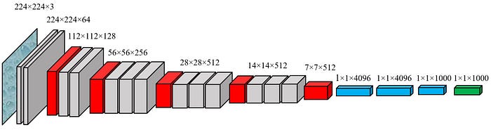
Custom Classifier

The “Custom Classifier” graph represents the custom classification part of the neural network that is added on top of the VGG16 feature extractor. This part of the network is trained on the specific dataset for the task at hand. It consists of a fully connected layer that reduces the 25088-dimensional input to 500 features, followed by a ReLU activation function, a dropout layer to prevent overfitting, another fully connected layer that reduces the 500 features to 102 classes, and a LogSoftmax layer to produce log-probabilities for each class. The final output is a vector of size 102, representing the probabilities for each class.

Device Selection

The line device = torch.device("cuda:0" if torch.cuda.is_available() else "cpu") is used to select the device on which the computations will be performed. If a CUDA-compatible GPU is available, it will use the GPU (cuda:0), otherwise, it will fall back to using the CPU. This ensures that the code can run efficiently on systems with a GPU while still being compatible with systems that only have a CPU. The print(device) statement outputs the selected device to the console.

Data Transformations

In the Image Classifier Project.ipynb notebook, we define transforms for the training, validation, and testing sets to preprocess the data before feeding it into the neural network. These transformations are crucial for several reasons:

1. Data Augmentation (Training Set): For the training set, we apply random transformations such as rotation, resizing, and horizontal flipping. This helps in augmenting the dataset, making the model more robust and capable of generalizing better to new, unseen data. By exposing the model to various altered versions of the same images, we reduce the risk of overfitting.
2. Normalization: For all datasets (training, validation, and testing), we normalize the images by scaling the pixel values to a range of [0, 1] and then applying a standard normalization using the mean and standard deviation of the ImageNet dataset. This ensures that the input data has a consistent distribution, which helps in faster convergence during training and improves the model’s performance.
3. Resizing and Cropping (Validation and Testing Sets): For the validation and testing sets, we resize the images to a fixed size and then crop the center. This ensures that the images are of the same dimensions as required by the pre-trained networks, allowing for consistent and accurate evaluation of the model’s performance.

By defining these transforms, we ensure that the data fed into the neural network is in the optimal format for training and evaluation, leading to better model performance and generalization.

Label Mapping

The cat_to_name.json file is used to map the category labels to the actual names of the flowers. This JSON file contains a dictionary where the keys are the integer-encoded category labels and the values are the corresponding flower names. By loading this file, we can convert the predicted category labels from the model into human-readable flower names, making the output more interpretable and user-friendly.

Build Your Network

In this section, we build and train a neural network for image classification using a pre-trained model from torchvision.models.

VGG

VGG (Visual Geometry Group) is a convolutional neural network architecture known for its simplicity and effectiveness. It consists of multiple convolutional layers followed by fully connected layers. VGG is a good choice for image classification tasks because:

• It has a simple and uniform architecture.
• It has been pre-trained on a large dataset (ImageNet), which helps in transfer learning.
• It achieves high accuracy on various image classification benchmarks.

Some good alternatives to VGG include:

• ResNet (Residual Networks): Known for its deep architecture and skip connections, which help in training very deep networks.
• Inception (GoogLeNet): Known for its inception modules that allow for more efficient computation.
• DenseNet (Densely Connected Convolutional Networks): Known for its dense connections between layers, which improve information flow and gradient propagation.

Dropout

Dropout is a regularization technique used to prevent overfitting in neural networks. During training, dropout randomly sets a fraction of the input units to zero at each update step. This helps in making the model more robust and reduces the risk of overfitting by preventing the network from relying too much on any single neuron.

Sequential

The nn.Sequential module is a container that allows you to build a neural network by stacking layers in a sequential manner. It simplifies the process of defining the network architecture.

nn.Linear

nn.Linear is a fully connected layer that applies a linear transformation to the incoming data. It is defined by the number of input and output features.

nn.ReLU

nn.ReLU is an activation function that applies the Rectified Linear Unit (ReLU) function to the input. ReLU introduces non-linearity to the model, which helps in learning complex patterns.

LogSoftmax

nn.LogSoftmax is an activation function that applies the logarithm of the softmax function to the input. It is often used in the output layer of a classification network to produce log-probabilities for each class.

Train Function

The train function is responsible for training the neural network. It takes the model, training data loader, validation data loader, loss criterion, optimizer, number of epochs, and device (CPU or GPU) as inputs. The function performs the following steps:

1. Moves the model to the specified device.
2. Iterates over the training data for the specified number of epochs.
3. For each batch of images and labels in the training data:

• Moves the images and labels to the specified device.
• Performs a forward pass through the model to get the output.
• Computes the loss using the specified criterion.
• Performs backpropagation to compute the gradients.
• Updates the model parameters using the optimizer.
• Accumulates the running loss.

4. Every print_every steps, evaluates the model on the validation data using the evaluate function and prints the training and validation loss and accuracy.

Evaluate

The evaluate function is responsible for evaluating the model on a given data loader. It takes the model, data loader, loss criterion, and device as inputs. The function performs the following steps:

1. Moves the model to the specified device.
2. Sets the model to evaluation mode to turn off dropout.
3. Iterates over the data in the data loader:

• Moves the images and labels to the specified device.
• Performs a forward pass through the model to get the output.
• Computes the loss using the specified criterion.
• Computes the accuracy by comparing the predicted classes with the true labels.

4. Returns the average loss and accuracy over the entire data loader.

Loading and Saving Checkpoints

Saving Checkpoints

Saving checkpoints is crucial for preserving the state of your model during training. This allows you to resume training from a specific point without starting over, which is especially useful for long training processes. Checkpoints typically include the model’s state dictionary, optimizer state, epoch number, and any other relevant information.

When to Save Checkpoints:

• During Long Training Sessions: Save checkpoints periodically to avoid losing progress due to interruptions.
• After Each Epoch: Save at the end of each epoch to ensure you can resume from the last completed epoch.
• Before Hyperparameter Tuning: Save the model before experimenting with different hyperparameters to have a baseline to revert to.

Loading Checkpoints

Loading checkpoints allows you to resume training from a saved state or use a pre-trained model for inference. This is useful for continuing interrupted training sessions or deploying a trained model without retraining.

When to Load Checkpoints:

• Resuming Training: Load a checkpoint to continue training from where it left off.
• Inference: Load a pre-trained model to make predictions on new data.
• Transfer Learning: Load a pre-trained model and fine-tune it on a new dataset.

Training the Model

Criterion and Optimizer

NLLLoss

criterion = nn.NLLLoss()

nn.NLLLoss stands for Negative Log Likelihood Loss. It is a loss function commonly used for classification tasks. This loss function expects the input to be log-probabilities (usually obtained from nn.LogSoftmax) and the target to be class indices. It measures the performance of a classification model whose output is a probability distribution over classes.

Adam Optimizer

optimizer = optim.Adam(model.parameters(), lr=0.003)

Adam (short for Adaptive Moment Estimation) is an optimization algorithm that can be used instead of the classical stochastic gradient descent to update network weights iteratively based on training data. Adam combines the advantages of two other extensions of stochastic gradient descent: Adaptive Gradient Algorithm (AdaGrad) and Root Mean Square Propagation (RMSProp). It computes adaptive learning rates for each parameter. The learning rate lr=0.003 controls how much to change the model in response to the estimated error each time the model weights are updated.

Train Function Parameters

train(model, train_loader, validation_loader, criterion, optimizer, epochs=1, print_every=40, device=device)

This line calls the train function to train the model. The parameters are:

• model: The neural network model to be trained.
• train_loader: DataLoader for the training dataset.
• validation_loader: DataLoader for the validation dataset.
• criterion: The loss function (NLLLoss in this case).
• optimizer: The optimization algorithm (Adam in this case).
• epochs=1: The number of times the entire training dataset will pass through the network.
• print_every=40: Frequency of printing training and validation loss and accuracy.
• device: The device (CPU or GPU) on which the computations will be performed.

Epochs

An epoch is one complete pass through the entire training dataset. During an epoch, the model sees each training example once and updates its parameters based on the computed loss. Training for multiple epochs helps the model to learn better by iteratively adjusting the weights.

Testing the Model

After training your model, it’s important to test its performance on a separate test dataset that the model has never seen before. This helps to evaluate how well the model generalizes to new, unseen data.

Evaluate Function

The evaluate function is responsible for evaluating the model on a given data loader. It takes the model, data loader, loss criterion, and device as inputs. The function performs the following steps:

1. Moves the model to the specified device.
2. Sets the model to evaluation mode to turn off dropout.
3. Iterates over the data in the data loader:

• Moves the images and labels to the specified device.
• Performs a forward pass through the model to get the output.
• Computes the loss using the specified criterion.
• Computes the accuracy by comparing the predicted classes with the true labels.

4. Returns the average loss and accuracy over the entire data loader.

Test Loss and Accuracy

Test Loss and Accuracy are key metrics used to evaluate the performance of a machine learning model on a test dataset.

Test Loss

• Definition: Test loss measures the error of the model’s predictions on the test dataset. It is computed using a loss function, such as Mean Squared Error (MSE) for regression tasks or Negative Log Likelihood Loss (NLLLoss) for classification tasks.
• Purpose: It helps in understanding how well the model generalizes to new, unseen data. A lower test loss indicates better model performance.
• Alternatives: Depending on the task, other loss functions can be used, such as Cross-Entropy Loss for multi-class classification or Hinge Loss for SVMs.

Accuracy

• Definition: Accuracy is the ratio of correctly predicted instances to the total instances in the test dataset. It is a straightforward metric for classification tasks.
• Purpose: It provides a simple measure of the model’s performance in terms of the proportion of correct predictions.
• Alternatives: For imbalanced datasets, other metrics like Precision, Recall, F1-Score, and Area Under the ROC Curve (AUC-ROC) are more informative.

Best Practices

1. Use Appropriate Metrics: Choose metrics that align with the problem’s nature. For example, use F1-Score for imbalanced classification problems.
2. Cross-Validation: Use cross-validation to ensure the model’s performance is consistent across different subsets of the data.
3. Monitor Overfitting: Compare training and test loss to detect overfitting. If the test loss is significantly higher than the training loss, the model may be overfitting.
4. Regularization: Apply regularization techniques like Dropout, L2 regularization, or early stopping to prevent overfitting.
5. Hyperparameter Tuning: Optimize hyperparameters using techniques like Grid Search or Random Search to improve model performance.

By following these best practices, you can ensure that your model is robust and performs well on unseen data.

Image Preprocessing

The process_image function preprocesses the image so it can be used as input for the model. This function should process the images in the same manner used for training.

Class Prediction

The predictor function uses a trained network for inference. It takes an image path and a model, then returns the top K most likely classes along with the probabilities.

Sanity Checking

To ensure the model makes sense, use matplotlib to plot the probabilities for the top 5 classes as a bar graph, along with the input image.

Deployment Guide

After development has been completed in the Jupyter IPython Notebook, we extract details into predict.py and train.py scripts for deployment. This document describes how to use the scripts in a real-life example, including their integration into a CI/CD pipeline and deployment to a production microservice. Additionally, it discusses the role of MLFlow in the CI/CD pipeline.

Using train.py and predict.py

train.py

The train.py script is responsible for training the image classifier model. It includes steps for loading and preprocessing data, defining the model architecture, training the model, and saving the trained model checkpoint.

predict.py

The predict.py script handles the prediction of image classes using the trained model. It includes steps for loading the model checkpoint, preprocessing the input image, and predicting the class of the input image.

CI/CD Pipeline

Continuous Integration (CI)

1. Code Quality Checks: Use tools like flake8 for linting and pytest for running unit tests to ensure code quality and correctness.
2. Automated Testing: Set up a CI service like GitHub Actions, Travis CI, or CircleCI to automatically run tests on the train.py and predict.py scripts whenever changes are pushed to the repository.
3. Model Training: Automate the training process by running train.py in the CI pipeline. Save the trained model checkpoint as an artifact for later use.

Continuous Deployment (CD)

1. Model Versioning: Use MLFlow to track and version the trained models. MLFlow can log parameters, metrics, and artifacts (model checkpoints).
2. Model Registry: Register the trained model in the MLFlow Model Registry. This allows for easy management and deployment of different model versions.
3. Deployment: Deploy the model to a production environment using a microservice framework like Flask or FastAPI. The microservice will load the model checkpoint and serve predictions via an API.

Role of MLFlow in the CI/CD Pipeline

1. Experiment Tracking: Use MLFlow to log experiments during the training process. This includes logging hyperparameters, metrics, and model artifacts.
2. Model Registry: Register the best-performing model in the MLFlow Model Registry. This ensures that the model is versioned and can be easily deployed.
3. Deployment: Use MLFlow’s deployment capabilities to deploy the model to a production environment. MLFlow supports various deployment targets, including Docker, Kubernetes, and cloud services.

Real-Life Example

Step 1: Setting Up the CI/CD Pipeline

1. Create a GitHub Repository: Initialize a GitHub repository and add the train.py and predict.py scripts.
2. Set Up GitHub Actions: Create a .github/workflows/ci.yml file to define the CI workflow. This workflow will include steps for installing dependencies, running tests, and training the model.

name: CI Pipeline

on: [push, pull_request]

jobs:
  build:
    runs-on: ubuntu-latest

    steps:
    - name: Checkout code
      uses: actions/checkout@v2

    - name: Set up Python
      uses: actions/setup-python@v2
      with:
        python-version: '3.8'

    - name: Install dependencies
      run: |
        python -m pip install --upgrade pip
        pip install -r requirements.txt

    - name: Run tests
      run: |
        pytest

    - name: Train model
      run: |
        python train.py

Step 2: Model Versioning with MLFlow

import mlflow
import mlflow.pytorch

# Inside the training function
with mlflow.start_run():
    # Log parameters, metrics, and model
    mlflow.log_param("learning_rate", 0.003)
    mlflow.log_metric("accuracy", accuracy)
    mlflow.pytorch.log_model(model, "model")

Register Model: After training, register the model in the MLFlow Model Registry.

# Register the model
model_uri = "runs:/{}/model".format(run_id)
mlflow.register_model(model_uri, "ImageClassifierModel")

Step 3: Deploying the Model

1. Create a Flask App: Create a app.py file to serve the model predictions using Flask.

from flask import Flask, request, jsonify
import mlflow.pytorch

app = Flask(__name__)

# Load the model
model = mlflow.pytorch.load_model("models:/ImageClassifierModel/Production")

@app.route('/predict', methods=['POST'])
def predict():
    data = request.json
    image_path = data['image_path']
    top_p, top_class = predict(image_path, model)
    return jsonify({'probabilities': top_p, 'classes': top_class})

if __name__ == '__main__':
    app.run(host='0.0.0.0', port=5000)

2. Dockerize the Application: Create a Dockerfile to containerize the Flask application.

FROM python:3.8-slim

WORKDIR /app

COPY requirements.txt requirements.txt
RUN pip install -r requirements.txt

COPY . .

CMD ["python", "app.py"]

3. Deploy to Kubernetes: Create Kubernetes deployment and service files to deploy the Docker container.

# deployment.yaml
apiVersion: apps/v1
kind: Deployment
metadata:
  name: image-classifier
spec:
  replicas: 2
  selector:
    matchLabels:
      app: image-classifier
  template:
    metadata:
      labels:
        app: image-classifier
    spec:
      containers:
      - name: image-classifier
        image: your-docker-image
        ports:
        - containerPort: 5000

# service.yaml
apiVersion: v1
kind: Service
metadata:
  name: image-classifier
spec:
  selector:
    app: image-classifier
  ports:
    - protocol: TCP
      port: 80
      targetPort: 5000
  type: LoadBalancer

By following these steps, you can effectively use train.py and predict.py in a real-life example, integrating them into a CI/CD pipeline and deploying the model to a production microservice.

To implement logging and monitoring for the deployed model, you can use a combination of tools and techniques. Here is a step-by-step guide:

1. Logging with Python’s logging Module

First, set up logging in your app.py file to capture important events and errors.

import logging
from flask import Flask, request, jsonify
import mlflow.pytorch

# Set up logging
logging.basicConfig(level=logging.INFO)
logger = logging.getLogger(__name__)

app = Flask(__name__)

# Load the model
model = mlflow.pytorch.load_model("models:/ImageClassifierModel/Production")

@app.route('/predict', methods=['POST'])
def predict():
    data = request.json
    image_path = data['image_path']
    logger.info(f"Received prediction request for image: {image_path}")
    try:
        top_p, top_class = predict(image_path, model)
        logger.info(f"Prediction successful for image: {image_path}")
        return jsonify({'probabilities': top_p, 'classes': top_class})
    except Exception as e:
        logger.error(f"Error during prediction: {e}")
        return jsonify({'error': str(e)}), 500

if __name__ == '__main__':
    app.run(host='0.0.0.0', port=5000)

2. Monitoring with Prometheus and Grafana

Step 1: Install Prometheus Client

Install the Prometheus client library for Python.

pip install prometheus_client

Step 2: Integrate Prometheus with Flask

Modify your app.py to expose metrics.

from prometheus_client import Counter, generate_latest, CONTENT_TYPE_LATEST

# Define Prometheus metrics
REQUEST_COUNT = Counter('request_count', 'Total number of requests')
PREDICTION_COUNT = Counter('prediction_count', 'Total number of predictions')
ERROR_COUNT = Counter('error_count', 'Total number of errors')

@app.route('/metrics')
def metrics():
    return generate_latest(), 200, {'Content-Type': CONTENT_TYPE_LATEST}

@app.route('/predict', methods=['POST'])
def predict():
    REQUEST_COUNT.inc()
    data = request.json
    image_path = data['image_path']
    logger.info(f"Received prediction request for image: {image_path}")
    try:
        top_p, top_class = predict(image_path, model)
        PREDICTION_COUNT.inc()
        logger.info(f"Prediction successful for image: {image_path}")
        return jsonify({'probabilities': top_p, 'classes': top_class})
    except Exception as e:
        ERROR_COUNT.inc()
        logger.error(f"Error during prediction: {e}")
        return jsonify({'error': str(e)}), 500

Step 3: Set Up Prometheus

Create a prometheus.yml configuration file.

global:
  scrape_interval: 15s

scrape_configs:
  - job_name: 'flask_app'
    static_configs:
      - targets: ['localhost:5000']

Run Prometheus with the configuration file.

prometheus --config.file=prometheus.yml

Step 4: Set Up Grafana

1. Install and run Grafana.
2. Add Prometheus as a data source in Grafana.
3. Create dashboards to visualize the metrics collected by Prometheus.

By following these steps, you can implement logging and monitoring for your deployed model, ensuring you can track its performance and detect any issues in real-time.

Conclusion

Convolutional Neural Networks have transformed how we handle classification tasks — offering remarkable accuracy once reserved for specialized research labs. But success isn’t just about hitting high accuracy metrics; it’s about deploying a model that’s robust, interpretable, and scalable to meet real-world demands. In this article, we showcased the entire process: from preparing your data and structuring your CNN architecture to fine-tuning and deployment considerations.

By following these steps and continuously iterating, you’ll be well-positioned to unlock the full potential of CNNs in your projects — whether you’re diagnosing medical conditions, powering autonomous vehicles, or building next-gen retail solutions. Remember, the ultimate goal of any deep learning initiative is to solve tangible problems and create meaningful impact for your organization and end-users. Armed with this knowledge, you’re ready to take the next step in implementing CNNs that truly make a difference.

If you’re hungry for more, remember that this entire tutorial is grounded in skills taught in Udacity’s AI Programming with Python Nanodegree. It’s a fantastic program for learning the foundations of deep learning with PyTorch and for building practical, resume-boosting projects like this Image Classifier.

For license details covering this content, please see:

https://github.com/udacity/aipnd-project/blob/master/LICENSE
https://github.com/jtayl222/aipnd-project/blob/master/LICENSE

Happy learning — and here’s to building something amazing!